Evaluating Wind Impact (Part III — Fuel Consumption and Emissions Evaluation)
By Kent Hawkins -- August 11, 2016“The best approach to understanding wind’s impact appears to be that properly structured ‘bench’ tests should be performed, and results made publically available, on actual fossil fuel plants under the full range of conditions experienced in balancing the effect of the presence of wind’s generation behavior.”
Part I on Tuesday and Part II yesterday focussed on the greater range of variations and the increased ramping levels caused by wind in short time intervals of a few minutes or less, and introduced some of the complexities involved in analysis of the impact of wind in an electricity system.
This post looks at the analysis of published fossil fuel consumption and emissions information and addresses two major issues:
(1) the questionable nature of the published information, and
(2) the questionable attempts by external analysts (those outside the information publisher organizations) using this information to determine the cause and effect relationship between wind production and fossil fuel consumption and emissions leading to the determination of savings with wind.
If information publishers were rigorous to the necessary degree in their determination, further analysis would be substantially reduced. This is not an easy task for either, and largely explains why it has not been done.
Published Fuel Consumption and Emissions Information
Unless you know otherwise, these should be viewed as estimates based on simplified assumptions, averages, aggregations over time and space, some measurements and limited algorithms that appear not to take fully into account the dynamic aspects of the ramping requirements as introduced in Parts I and II.
Fuel and emissions calculations that start with electricity production data and from there calculate back to arrive at results for these based on static-oriented generation plant efficiencies and other simple assumptions are particularly suspect. [1]
There appears to be a broadly accepted practice of using such simplified approaches. The advantage to this is that it may be somewhat useful in making rough comparisons between jurisdictions and time frames if the same method is used, but not in determining absolute values.
Factors Impacting Fossil Fuel Consumption and Emissions
Examples of factors affecting fossil fuel consumption and emissions include:
- Changes in the generation plant fleet profile at any point in time. This also includes scheduled and unscheduled maintenance with might remove/add plants at different efficiency capabilities. An interesting example could be sometimes running the more efficient CCGT as OCGT gas plants. Also included would be plant closures and new plant implementations within the time frame studied.
- Changes in net interchange activity. Although many jurisdictions will have lower levels of activity than the BPA, even levels at a small per cent of the total generation will be notable. Further, it is important to separate the export/import flow except perhaps at short time intervals, to properly understand their impact, which can be considerable even at low net For an example see the paragraph entitled Power Imports: The Missing Piece at OVERBLOWN: Getting to the Facts on Emissions .
- Changes in quality of fossil fuel used from time to time. This is more obvious with coal, but caloric content per unit volume of natural gas can also vary.
- Changes in level and nature of economic activity.
- Grid events that may be responded to differently from time to time depending on the availability of generation plants suitable to the task at hand.
- Balancing activities that take place at regional levels within a grid, versus assuming balancing on total grid aggregate levels.
Statistics General
Statistical approaches are questionable because the real world events with wind present do not conform to a normal distribution, which is typically implicitly assumed. An important aspect of this is the assumed number of outliers for 3-4 standard deviations is very small (0.03-0.01 per cent of the total respectively), but this is not what happens with wind present in electricity systems.
Assuming that any notable ‘outliers’ would be as expected in a normal distribution contributed considerably to the failures in financial institutions and markets in recent history.
Table 1 summarizes the data shown in Part II to illustrate the large number of ramping events exceeding a range of standard deviations, loosely termed ‘outliers’. In this table, ‘Load and Wind Combination’ is ABS(L-W) – ABS(L), where ABS is the absolute value, as explained in Part II.
Table 1 – Load and Wind Combination Ramping Events versus Normal Distribution Expectation for January to June 2015
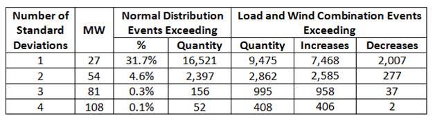
Comments on Table 1:
- For total events see Part II, Tables 1 and 2.
- Although the load and wind combination shows fewer events exceeding one standard deviation overall, in the range of greater than two standard deviations, there are a significantly greater number of them than is expected for a normal distribution. This is a notable number of surprises.
- A questionable use of statistics is to imply a single standard deviation (27 MW in this case) represents the effect of wind, perhaps to suggest that it is very benign. See National Renewable Energy Laboratory report (Figure 3), and commented on here (in paragraph commencing with ‘Figure 3 should have displayed…’)
Correlation
Some analyses rely on these, for example, to determine a cause and effect between wind production and reported emissions. If so, it is necessary to separately demonstrate that no other factors are influencing emissions production, even if all other factors appear to be accounted for.
For numerical correlation to demonstrate cause and effect, the simple approach of a time series plot of the two variables can be used. The degree to which the two variables do not match in timing and proportion (if the two variables are different entities) will indicate how much other factors are at play. Paul-Frederik Bach, who was a senior executive in the Danish electricity system, illustrates this clearly in “Wind Power Variations are exported” in the third chart on page 3. This is reproduced with permission as Figure 1.
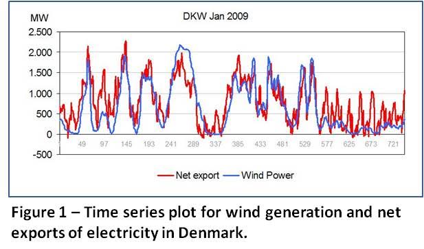
Figure 1 shows wind production and net exports in the Danish system for one month. Actual exports would be a better measure, but this information may not be readily available. The close tracking in timing for much of the period up to about point 550 supports the case for a close cause and effect relationship between the two time series variables. A negative correlation would show a mirror image. Proportion is not a factor here because both variables are the same entity – electricity.
There are some other factors at play in this illustration – in the ranges 0-50, 75-100 and 250-300. After about 550, with little or no wind present for days, exports are drawn from other resources, for example (1) from within Denmark, or (2) as Denmark is a conduit between Norway/Sweden and other European countries, it is acting as a pass-through. [2]
I have seen a claim of “mission accomplished” using such a chart that showed only the slightest correspondence between wind generation and emissions. It really showed that many other factors not accounted for were involved. So do not accept a claim of a cause and effect relationship for two time series variables in any analysis that does not clearly demonstrate this with a plot as shown in Figure 1. In addition, the source of the data, especially emissions data, must also be questioned.
Regression
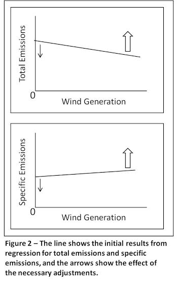
Regression based on a plot of emissions versus wind production over a period of time is another approach used to analyze a jurisdiction with wind installed. The results typically show a decline of emissions as wind increases. If specific emissions are used then this will increase as wind increases. In general, this is inconclusive because of the nature of the emissions data on which it is based, as discussed, and many other factors that might affect emissions, as described above.
Further, as there are periods of no wind electricity production, the implied assumption is that the no-wind-at-the-moment case is the same as it would be if there was no wind installed in the electricity system. Here is one possible illustration of the difference. During the periods of no-wind-at-the-moment, CCGT plants could operate in their normal mode and the more flexible OCGT plants may now be employed at some level of loading to respond to the reappearance of more wind generation.
These OCGT plants (or CCGT plants in OGT mode) would not be required in the no-wind-installed case, which represents the proper baseline. The additional use of OCGT in the no-wind-at-the- moment case would produce more emissions and higher specific emissions than the no-wind-installed case, which would lower the proper start point on the graph.
During periods when wind is generating a notable amount of electricity, the underlying data is not capturing the full dynamic effect of the continuous ramping imposed, as discussed in Part II. Both the emissions and specific emissions should be increasingly higher as wind increases than plotted using the published data, probably to a greater degree than the adjustment for no-wind-at-the-moment. [3]
Both considerations will contribute to rotating the graphs considerably counter-clockwise, showing a much less attractive view of total emissions and specific emissions results for wind as shown in Figure 2. [4] The size of the arrows is intended to show the likely degree of change.
Now add back in all the considerations of questionable emissions data and other factors influencing emissions as discussed above.
Conclusions
It is very difficult for any theoretical analysis to adequately deal with all the issues touched on here, plus many others not identified.
The best approach to understanding wind’s impact appears to be that properly structured ‘bench’ tests should be performed, and results made publically available, on actual fossil fuel plants under the full range of conditions experienced in balancing the effect of the presence of wind’s generation behavior. [5] It is reported that something like this has been done by KEMA, an international consulting firm based in the Netherlands, but the results are not publically available. [6]
Such tests would likely still not reflect the effects of any total grid aggregation. However, as grids are often balanced regionally, the effects of aggregation would likely be relatively small compared to the test results, and would have the benefit of better isolating the effect of wind.
I expect the ‘bench’ test results would be adversely surprising for wind, which might explain why this has not been done.
—————————
[1] Based on a quick review of my previous posts, here are some references for what I have found on this issue.
- Primary Energy Consumption Part II http://www.masterresource.org/energy-sources/primary-energy-electricity-ii/ See endnote 1.
- Where Wind Studies Go Wrong: Cullen in AEG (Part II) http://www.masterresource.org/emissions-reduction-wind/where-wind-studies-go-wrong-part-i/. See links to IEA and Irish System in the Questionable Data
I have attempted at least twice to obtain details of how fossil fuel consumed and emissions are determined for electricity systems in separate jurisdictions. In both cases my request was not responded to. So if anyone can provide detailed descriptions of how any jurisdiction does this, this information would be welcome. In summary, in using this data in analyses you should ensure you fully understand how it was developed.
[2] Denmark’s case is fairly complex. For more detail see the MasterResource series “Peeling Away the Onion of Denmark Wind” at http://www.masterresource.org/false-claims/denmark-part-i-intro/ .
[3] Further, some CCGT plants may have to operate in OCGT mode to meet flexibility needs. The assumed emissions for the CCGT plants may be based on the normal CCGT specifications at all times.
[4] Total emissions are in tonnes and likely for the total electricity system. Specific emissions, tonnes per MWh, may be for the total system or for identified generation plants that are balancing wind.
[5] The actual specifications for the tests would require considerable development. As an example of some of the considerations are the following four general scenarios: (1) a constant load baseline, (2) responding to up and down steady trends simulating twice daily intermediate and peaking demand, (3) a straight frequency regulation role, and (4) finally to the addition to a wind component in cases 2 and 3.
[6] It is reported that KEMA showed that the cycling of fossil fuel plants from a normal full load to reduced load and back to normal over one hour resulted an increase of more than 1% fuel consumption over operating normally for the same period. See paragraph 4.a Cycling at http://www.clepair.net/windSchiphol.html. This means that this limited cycling of fossil fuel plants increases emissions over their steady state condition, and it is reasonable to expect that continuous frequent cycling would increase this even more. This cycling already occurs in load following in the short term and the same, but to a greater degree, when balancing wind. Note that when cycling less electricity is produced over the hour than normal, steady state. This strongly suggests that the fuel consumption and emissions increases with the presence of wind. So simply relating emissions to electricity generation with simplified efficiency assumptions is a questionable approach to analyzing wind emissions performance.
[…] I sets the stage with basic information as context for more detail in Part II. Part III addresses the issues in (1) the published information available for analysis, and (2) the use of […]
In this three part series, Kent Hawkins has told more than a cautionary tale about the difficulties involved with claiming that wind technology is an effective way of avoiding CO2 emissions in the production of electricity. For years, the various wind trade associations and their revolving door allies in government organizations like the National Renewable Energy Lab, have touted the notion that wind output displaces carbon fueled generation on a one to one, kWh to kWh basis, taking refuge in the simplistic notion that because demand and supply must always be in perfect balance, more supply of wind must result in a correspondingly less supply of mainly fossil fired generation (given the relative dearth of hydro and nuclear power around the nation and the globe). These claims have been accepted as truth by mainline media, a flotilla of politicians and their policy wonks, virtually all electricity regulatory commissions, and even, superficially, organizations like FERC and the USEIA. All of this has been abetted by economists who don’t know the difference between a kWh and nosegay; in report after report, economists continue to perpetrate the fraud that wind is as respectable an energy source as any other–and quite capable of displacing fossil fuel production and their associated emissions.
Over the last decade, some have begun to question this idea, however, doing so in the ways Kent has described in this essay, using half baked analysis, demonstrably incomplete data, and sophomoric statistical tools. The most comprehensive of these analyses claim that wind only reduces about half of the emissions claimed by wind proponents. Which, for the likes of Greenpeace, the Sierra Club, and even AWEA, is still good news for the planet. However, when challenged to show even a correlation between the 50% wind savings which these folks claim and a corresponding reduction in fossil fuel reductions, the challenge is met with a wall of silence. Because, uh, their is no such correlation that can survive any scrutiny.
What Kent does here is show that both the unscience of AWEA and the NREL and the merely bad science of the wind 50 percenters have absolutely no value in explaining whether or how much wind can reduce overall CO2 emissions in the production of electricity. Because of the complexity involved combined with a heavy veil of trade secrecy that makes transparent evaluations nearly impossible, no one knows the answer to this question.
Hence there is genuine nutcasery behind governmental policy that privileges wind technology and its related renewables du jour and provides it with hundreds of billions of dollars from the public treasury because there is no veridical evidence that wind avoids any overall emissions in the production of electricity. As Kent shows here, and as he has shown elsewhere over the years, most of the evidence that does exist suggests wind output in many jurisdictions is responsible for increasing CO2 emissions beyond what would have been the case without any wind at all.
Why is this?
Consider the basic facts of wind performance that should be known to those familiar with the articles posted on Master Resource over the years. The technology delivers an annual average of between 15 and 30 percent of its rated capacity to a grid; 60 percent of the time, it is less than this. Around 10 percent of the time, wind produces nothing. Its output peaks at times of lowest demand and is lowest at times of peak demand. Whatever it does produce is always jittering–at the cube of the wind speed along a narrow windspeed range.
I wish Kent had written a preamble that dealt squarely with why wind is such a dysfunctional lummox. As physicists and knowledgeable engineers know, the dilute energy from the wind is converted by a well understood formula–w=1/2 rAv3, where w is power; r, air density; A, rotor density; and v is wind speed. The main driver in the equation is the V3, which dictates that any output must be a function of the cube of the wind speed at each wind speed interval throughout the windplant’s rated capacity. Typically, a wind turbine does not begin producing electricity until the wind speed reaches 8 mph. And it reaches its rated capacity when the wind speed hits 33 mph (wind speeds beyond this don’t change the output level; if wind speeds hit ~53 mph, the turbine is shut down to prevent damage).
Accordingly, small differences in wind speed lead to large differences in “power.” If the wind speed doubles, wind “power” increases by a factor of eight. For example, an output at 10mph, a small fraction of a wind project’s installed capacity, is doubled when the wind speed hits 12.6mph. And vice versa in reverse, up and down, throughout the entire range of the wind plant’s rated capacity, from zero to the maximum. I submit that this minute by minute variability, one that is random, unpredictable, uncontrollable (unless the wind machine is shut down or not yet producing output) that makes wind le mauvais garcon of modern power generation: for whenever it generates output, it is continually subverting the grid’s prime directive of keeping supply perfectly matched with demand. The geometric nature of its skittering output, up and down the entire range of its rated capacity at the cube of the wind speed along a narrow wind speed range, requires that it be continuously shadowed, in yin/yang fashion, by conventional generation that must existentially operate in a less efficient manner. Even if we could predict wind output (and we cannot), its fluttering nature would continue to induce substantial inefficiencies, which around the world would, as has been the case for decades, since most conventional generators are either coal or gas-fired, induce in turn substantial heat rate penalties, with all this implies in terms of fuel savings and emissions….
And the more wind generation, the greater the variable range. A 200MW windplant is less problematic (though still worrisome) than one rated at 1000MW. This is why, if one is a consumer of electricity, higher wind capacity factors are undesirable, for they increase the financial cost of wind integration and substantially increase the risks to grid security.
The relentless volatility of wind output as mandated by formula and acted upon by the random gustiness of wind (which is even more pronounced at higher altitudes) in my view largely explains the frequency of wind variations that I believe are the central revelation in Kent’s post. Given the formula for wind energy conversion to “power,” this frequency variation is neither surprising nor unexpected. Rather, it is the existential nature of wind behavior. As such, wind volatility must always subvert the grid’s primary mission, in the process inducing ubiquitous inefficiencies throughout the grid system, including frequency control and transmission regulation.
None of this should diminish the importance of Kent’s general thesis. He has also put in play many of the factors that must be properly defined, gauged, and epistemically coordinated with other factors in order to achieve better explanations. As he points out, using “averages” that smudge important distinctions and blur reality is problematic at best and, at worst, disingenuous. And making claims about results that aren’t independently verified from a variety of checkpoints and perspectives is little more than methodological sophistry.
I hope Kent’s series here gets wide distribution, for it can serve as a new platform on which honest people in search of honest answers on behalf of better ideas can firmly stand.