The Calculator: Fossil Fuel Consumption, CO2 Emissions, and Costs with Wind (Part I)
By Kent Hawkins -- November 29, 2010[Editor note: Kent Hawkins has been at the forefront of devising a model (the Calculator) to estimate the lost wind-related emission reductions due to the fact that backup fossil-fuel generation (to firm wind) must operate less efficiently. This two-part series (today and tomorrow) provides Mr. Hawkins’ latest thinking. While technical, the Calculator is a very important line of analysis that will continue to be revised by its open-minded author. So critical comments are especially welcome.]
There is no convincing proof of the ability of utility-scale wind electricity generation to provide any of the incredible benefits claimed for it. In light of the massive costs (hundreds of $billions) of the extensive implementations projected by some governments, and equally large changes to electricity grids required to support wind’s ineffectiveness, it seems reasonable to expect that such claims be properly substantiated beforehand.
Among the more important claims are fossil fuel and CO2 emissions reductions. In the absence of (1) any verification of these, ignoring of course the many uncritical testimonials by government bodies, environmentalist organizations and the media, and (2) the necessary public information to objectively analyze wind’s performance, the Calculator was developed as an interim tool to assist in understanding some of the realities of integrating wind into electricity systems. It shows the fossil fuel consumption, CO2 emissions and associated costs, based on a range of input factors.
This update is based on feedback from the Calculator series and comparisons with studies involving some level of actual results by Bentek and le Pair and de Groot. (A copy of the Calculator can be obtained here). There are no changes to the approach taken, but improvements have been made, including a better user-interface. Note that input should be entered only in cells that are outlined or by using the provided sliders. Other cells contain calculated amounts or references.
Critics have charged that the Calculator is not based on any production data to support the results reported in the Calculator series. But, this misses the point. Considering that there is not sufficient, appropriate data available publically to permit a comprehensive analysis, the calculator expresses a working hypothesis based on the important factors that bear on wind integration:
- Impact of wind volatility on fossil fuel plants required to balance wind production
- The need to introduce fast-reacting but less efficient gas plants into the generation portfolio
- Focus on the effects of the intertwined nature of wind plants and fossil fuel plants versus macro analyses, for example, at the country or state level
- Seasonality of wind production
- Consideration of the likelihood that some fossil fuel plants in the wind-balancing role may be able to operate “normally”, for example in periods of low wind production, including no wind conditions.
So the Calculator does not “prove” that wind plants increase CO2 emissions but shows the impact of a number of considerations. To illustrate this, it can be used to show what is often claimed by wind proponents. To do this, set the parameters so that there is (1) no efficiency loss in balancing fossil fuel plant and hence no increased fossil fuel consumption and CO2 emissions per MWh, (2) no change in capacity factor of the wind-balancing fossil fuel plants, and (3) there is no need to introduce more fast-reacting but less efficient gas plants (known variously as OCGT, SCGT and CT) into the plant portfolio.
The point is that the Calculator should:
- Cause users to think about the many factors involved in the integration of poor performing, unreliable and intermittent wind plants when doing their own analyses or reviewing others.
- Be seen as a way of quickly seeing the effects of varying these factors. It saves a lot of calculations, and provides a means of testing the sensitivity of each.
In other words, the Calculator is a framework within which to think about these considerations. As an example that is transferable from every day experience, does your car use less gas per mile driving at a relatively steady speed on the highway compared to the stop/start, speed-up/slow-down overall slower speeds of city driving? This can be applied to the effect on gas plants balancing wind’s intermittent behaviour, versus their running on a relatively steady basis as they were intended. See Part II for a discussion of newer gas plant types.
The latest version also calculates the cost per tonne of CO2 emissions saved or increased, depending upon input parameters. The first is the cost of CO2 mitigation and the second is, in effect, the cost of actually subsidizing CO2 emissions when wind plants cause their increase.
Heat Rate Penalty
An important part of the Calculator is the relationship between the reduced efficiency of the wind-balancing fossil fuel plants as a result of having to mirror wind’s random, intermittent variability (involving the full range of wind capacity) and the amount of fossil fuel consumed and CO2 emissions produced as a result.
The first issue that must be addressed is the heat rate penalty experienced over time (the Calculator assumes a year) by the fossil fuel plants in the wind-balancing role. This is not an instantaneous value, which might be observed at a point in time. It should also not be interpreted as a heat rate penalty due to continuous, “normal” operation at a reduced efficiency level. Nominally, I choose a heat rate penalty of 20%, which is intended to incorporate all the considerations. The Calculator provides for a range of 0-30% which should be adequate.
If you are satisfied that this is a reasonable heat rate penalty, but less satisfied that this should apply to all plants operating in the wind balancing role you can alter the heat rate penalty by a factor of 0-100%, which is in effect representing the amount of time that a heat rate penalty applies. Examples, requiring this would be: (1) a wind regime where the wind production rarely if ever reaches 100%, and (2) the case when wind production is zero to very small for relatively lengthy periods of time. Zero percent means there is no heat rate penalty and 100% means that the selected heat rate penalty value is used unaltered. Within gas plants, likely only the CCGT plant heat rate should be adjusted in this way. The use of two factors is a bit redundant, but it serves to make the two considerations explicit.
Figure 1 shows the effect on CO2 emissions for the case of CCGT alone in a wind balancing role (the question of the feasibility of this is not addressed) and also with the introduction of OCGT, for a range of heat rate penalties for CCGT from 0 to 20% (the x-axis). The heat rate penalty for OCGT is set at 20%. The ratio of CCGT:OCGT for low and high wind periods used is 70:30 and 30:70 respectively.
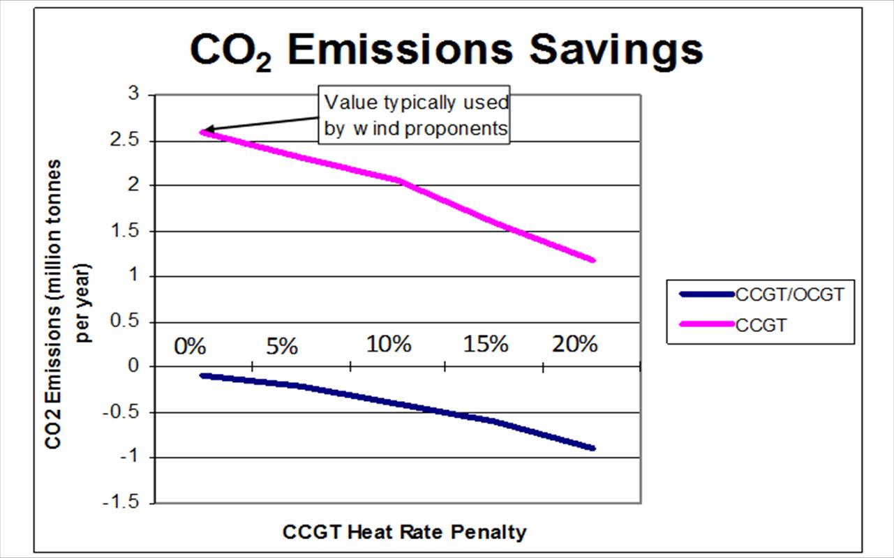
Figure 1 – Using only CCGT plants for wind balancing, there are CO2 emissions savings. Once OCGT plants are introduced into the wind-balancing mix, CO2 emissions savings become negative, that is, emissions are increased. At the CCGT:OCGT mix used, even at no heat rate penalty for CCGT plants, emissions are still slightly increased by about 100 tonnes per year.
The introduction of OCGT (alternatively CCGT operating as OCGT) has a dramatic effect. It is arguably necessary to provide the capability to respond to wind’s volatility, but is almost always overlooked in analyses of wind and CO2 emissions.
The cost per tonne of CO2 emissions for these conditions is shown below in Figures 2 and 3.
Required Fossil Fuel Plant Capacity
The Calculator does not show the capacity of the fossil fuel plants that are dedicated to wind balancing, and assumes the fossil fuel plant capacity for this purpose is available. In a specific case if it is not available, then additional plants must be built, but this does not affect the calculator results. It is a capacity planning matter. It should be noted that capacity in excess of requirements without wind must be available for wind balancing. Germany provides evidence of this here and here at slide 13. For a capacity planning purposes, capacity credit shows a statistical value over time to meet some level electricity system reliability. As an aside, capacity credit values for wind for electricity system reliability less than 99% should be suspect.
In determining CO2 emission costs per MWh of wind production, the full levelized costs of the wind balancing fossil fuel plants are used, whether it is new build or existing.
Cost of CO2 Emissions Mitigation/Subsidization
For details see the Costs tab in the Calculator. Note that there is an adjustment parameter for fossil fuel plant capacity factor, which is left there so the effect of varying it can be more easily seen. Unless the user wants to vary this, care should be taken that this is set at 100%. For ease of reference, the value set is shown in the User Interface.
The levelized costs used are those found in the DOE EIA’s Annual Energy Outlook 2010. Note that capital costs component have been subsequently adjusted upwards by the DOE EIA here, which shows increases in capital costs (overnight) of 21% for onshore wind, 49% for offshore wind, 25% for coal, 39% for OCGT and -3% for CCGT.
If the presence of wind reduces CO2 emissions the costs are mitigation costs. If wind increases CO2 emissions then the costs are actually subsidizing this unintended consequence.
Figures 2 shows the Calculator results for CCGT heat rate penalties from 0-20%.
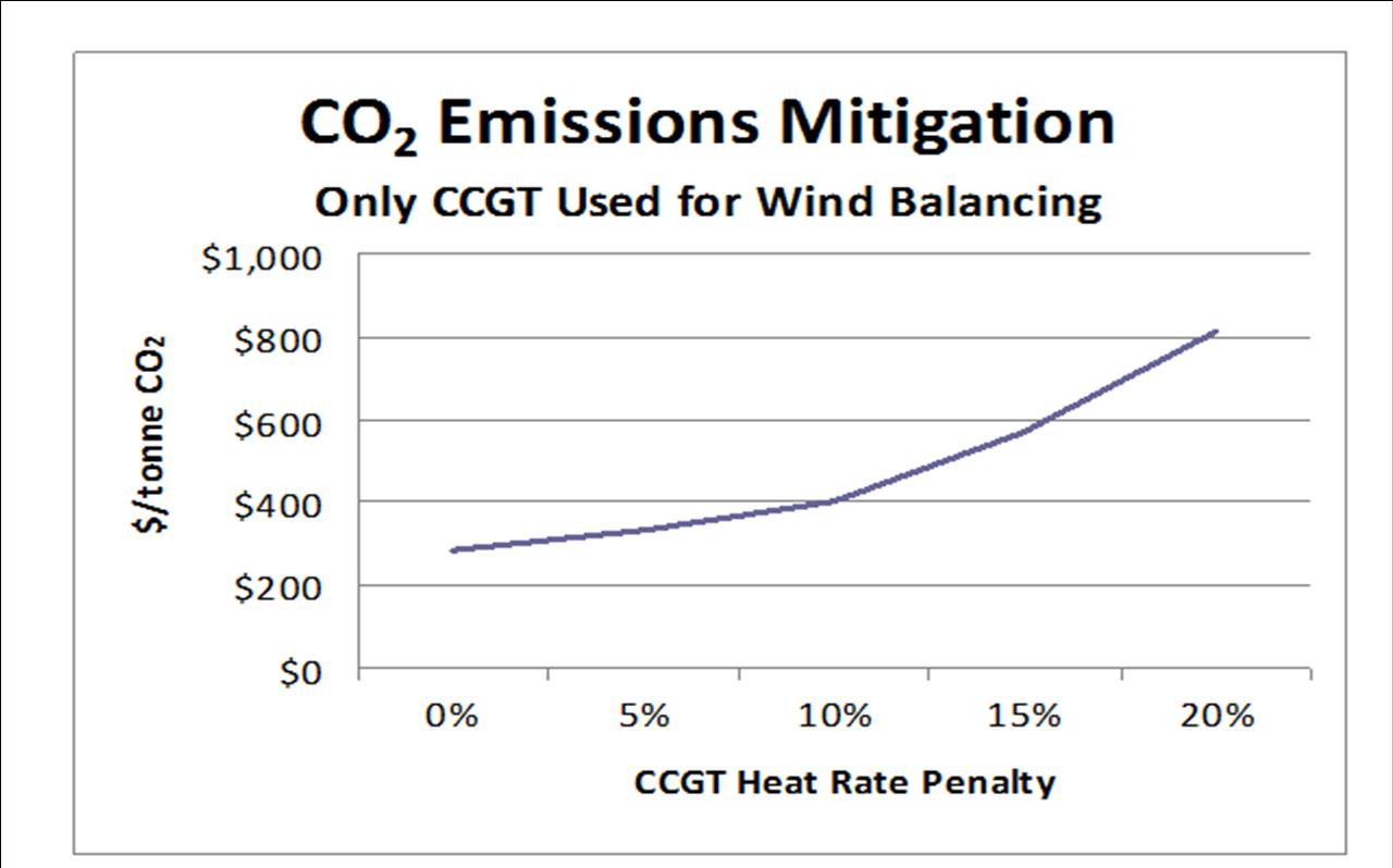
Figure 2 – Costs of mitigating CO2 emissions with wind assuming CCGT alone is used for wind balancing. A heat rate penalty of 0% is a typical condition for CO2 emissions savings used by wind proponents and produces savings of 2.6 million tonnes of CO2 per year. At this point, the Calculator shows a cost of $284/tonne CO2.
The cost per tonne increases with increased CCGT heat rate penalty because the CO2 emissions savings decrease and the costs increase slightly due to increased variable Operations and Maintenance (O&M) costs for the CCGT plants. Remember the heat rate penalty shown is an annual average, not an instantaneous value, which will be higher.
As an aside, and explaining some CO2 mitigation costs that may be claimed, if coal plant production is assumed to be displaced by wind acting alone, and without any heat rate penalty for the wind-balancing coal plants, the costs are $100 per tonne CO2.
In any event all these costs are multiples of those experienced in emissions trading markets in Europe and the US.
When OCGT plants are added to the mix, emissions savings can become negative. The associated costs become a subsidization of the production of CO2 emissions with values as shown in Figure 3.
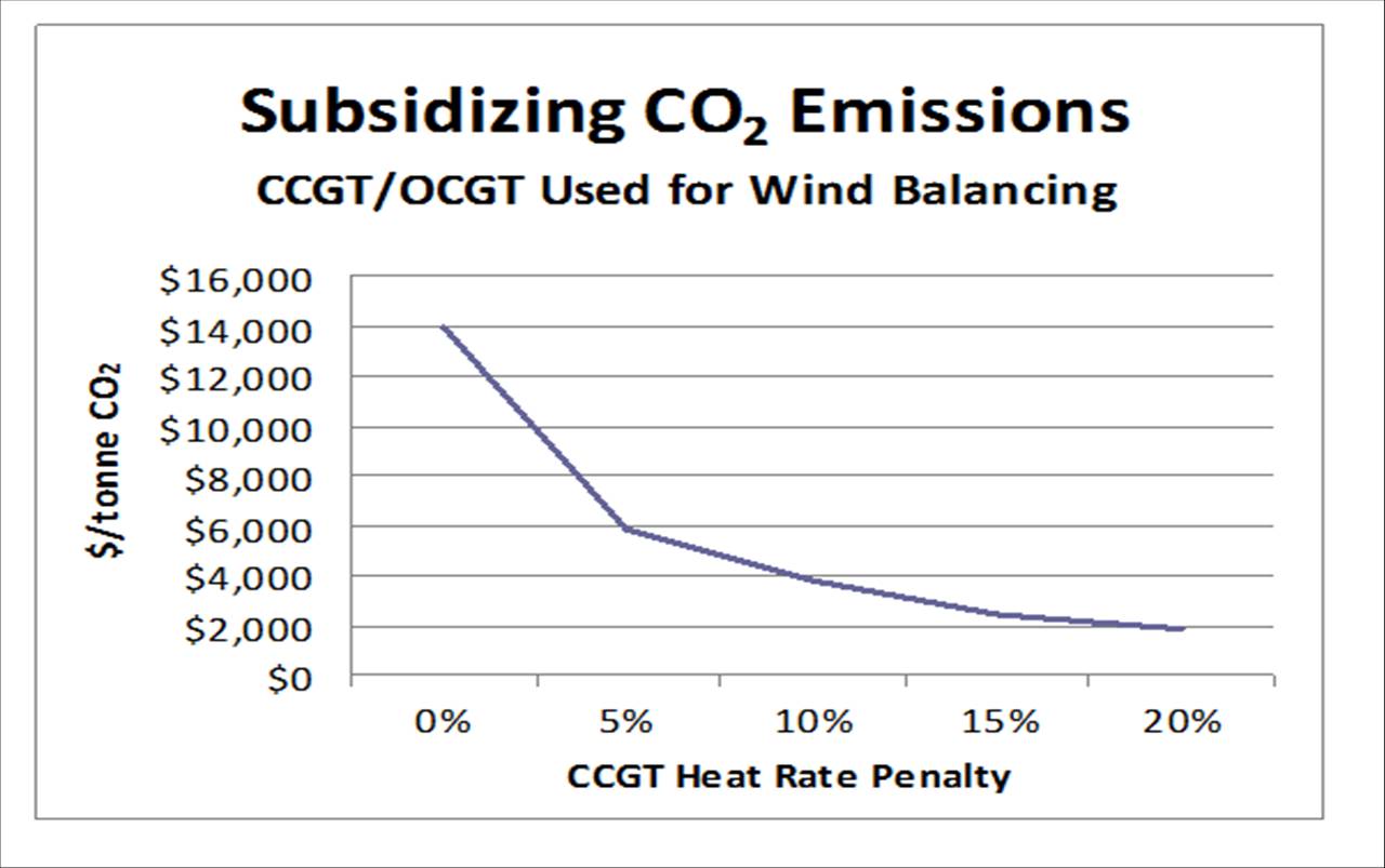
Figure 3 – Realistically OCGT plants will be needed to balance wind’s continuous volatility. Assuming a CCGT:OCGT mix for low and high wind periods to be 70:30 and 30:70 respectively shows substantially higher costs than assuming CCGT alone, due to the lower efficiency of OCGT gas plants. The costs at 0% CCGT heat rate penalty are the highest because CO2 emissions savings have just turned into a small increase of 100 tonnes per year. The subsidization cost rate decreases as the CO2 emissions increase due to emissions increasing faster than costs.
Although subsidization costs decrease with increased CCGT heat rate penalty, these costs remain very high. In summary, the Calculator shows that jurisdictions with such conditions are paying substantially in terms of actually subsidizing the creation of CO2 emissions. In your country state or province, look for the implementation of OCGT (also known as SCGT or CT) plants. As an alternative, but less discernable situation, especially with small wind penetration, the operation of CCGT plants in OCGT mode may be occurring.
Part II describes the Calculator in more detail, and provides information to assist in countering wind proponent claims.
Notwithstanding the limitations of the Calculator, any realistic choice of input parameters for it shows that the pursuit of policies providing incentives for the implementation of utility-scale wind plants is a futile solution for reducing the use of fossil fuels and CO2 emissions. The required expenditure of the large amount of national wealth, in the order of many hundreds of billions of dollars, is folly. Further exacerbating the financial aspects is the inherent potential equity euphoria and securitization of such programs. This, plus the diversion of human resources in government and industry otherwise needed to provide effective solutions for present and future electricity needs, will be seen as a critical lost opportunity to the detriment of future generations in all countries.
—————————————-
Update: The Calculator link has been changed to provide for separate access for Excel 2003 and 2007. Some graphics on the User Interface spreadsheet did not display correctly. I apologize for any inconvenience this has caused. (Kent Hawkins January 15, 2011)
Why would anyone except a wind developer and their acolytes at the National Renewable Energy Lab assume that a wind/CCCC pairing, even at small levels of wind penetration, would not affect the CCCC plant’s efficiency by increasing its heat rate? Combined cycle plants are designed to run continuously at a steady level without much operational toggling–which is why open cycle plants are deployed to engage wind’s relentless volatility. To the extent that combined cycle gas units alone balance wind flutter, the more wind, the more inefficient the CCCC plant–to the point of increasing overall CO2 emissions.
Moreover, readers should keep in mind that in the real world across much of the US, it is coal plants that now overwhelmingly balance wind flux; natural gas usage, although perhaps the best pairing for wind in terms of any CO2 offsets, would have to be increased significantly in order to achieve routine circumstance. Even then, it would be dicey if wind displaced a coal plant to be balanced by the gas plants, for, as Kent shows, even here, if the balancing were done by open cycle gas units, which would be overwhelmingly the case, more CO2 would be emitted as a result.
Although I look forward to Part II, perhaps I might suggest that a concomitant inquiry be made measuring overall fuel use. As Kent’s work suggests, CO2 emissions, which are accounted for in highly statistical and imprecise ways, are only part of his calculation. The other part predicts that wind volatility can offset very little overall fossil fuel consumption–and in some cases may actually increase that consumption.
In examining wind activity in Texas and Germany, in Denmark and Colorado, I cannot find any causal relationship between increased wind penetration and reduced fossil fuel consumption. Any reductions are much more likely caused by reductions in demand, whether influenced by the general economy or increased conventional plant efficiency–or increases in capacity fuels, such as hydro or nuclear that infill reductions in coal/natural gas.
Here’s a link to a related post on my blog:
Video: Power company official reveals that wind farms are ‘in fact, creating emissions’
http://algorelied.com/?p=3904
The video features Todd Wynn of the Cascade Policy Institute who was told by a Bonneville Power Administration staffer that wind farms “created emmissions”.
Don’t miss the comments where a Bonneville Power official tries to put that Genie back in the bottle, and Wynn retorts with more data.
The Calculator: Fossil Fuel Consumption, CO2 Emissions, and Costs ……
Here at World Spinner we are debating the same thing……
[…] The Calculator: Fossil Fuel Consumption, CO2 Emissions, and Costs with Wind (Part I) – Kent Hawkins at MasterResource […]
There is lots of wind data for Ontario Canada. How your calculator would work here I don’t know.
http://ontariowindperformance.wordpress.com/2010/09/24/chapter-3-1-powering-ontario/
Here is a link to the first study.
http://windconcernsontario.wordpress.com/2010/06/18/watts-up-with-the-wind-in-ontario-2010/
The data for Ontario Canada is quite complete. There may be minor omissions, but it should provide an interesting test case. Both articles provide links to the source data.
Cheers!
Thanks, Klockarman. Master Resource some months ago posted Eric Lowe’s fine piece about wind and CO2 emissions along the BPA:http://www.masterresource.org/2010/07/northwest-windpower-problems. He had acknowledged Todd Wynn’s assistance. Afterward, BPA’s chief spinner, Doug Johnson, as he does in the news documentary, attempted damage control. He failed. Do read all the comments, including mine, Kent Hawkins’, Don Hertzmark’s, and Lowe’s, who pointed out that BPA was only following the law.
My hero in all this is Deb Malin, the BPA official who simply blurted out the truth in response to the question of whether or not wind abates carbon emissions. As I had said, she’s probably now in some purgatorial gulag at BPA–and not allowed to go near any media.
Meanwhile, Johnson works hard to polish the wind apple for media, as the video here shows. The reality is that even in Oregon, with the best circumstance for wind with so much hydro, wind technology remains dysfunctional, causing all systems to work much more inefficiently. The amount of wind penetration is pressing the limits of hydro to compensate for its increasing volatility, which is why the desire for new natural gas units. And the consequence of this is embedded in Kent’s current article.
WillR
The Calculator runs in this post just happen to be for the projection of wind implementation in Ontario for 2015 by the OPA, that is 3,200 MW.
In response to a point made in Jon Boone’s first post, the fossil fuel use can be seen by downloading the calculator (link provided in the third paragraph of the post) and looking near the bottom of the page under the User Interface tab.
I have been asked to clarify the statement, “As an aside, capacity credit values for wind for electricity system reliability less than 99% should be suspect.”
Capacity credit for wind varies depending on (1) penetration of wind in terms of electricity production, and (2) assumptions made for the statistical analysis providing the expectation of wind availability at peak demand. Some reported capacity credit values assume an electricity system reliability of only about 90%. This yields an unrealistic wind capacity credit of about 20% for Germany, whereas the German Energy Agency, dena, reports wind capacity credit at about 8%, using a system reliability level of 99%.
Capacity credit for wind increases non-linearly as wind penetration is reduced. As wind penetration approaches zero, wind capacity credit approaches the level of wind capacity factor, which is usually in the high twenties in percentage terms. Intuitively this latter point makes sense, because the failure of wind to produce at very low penetrations is not critical.
The intent here is to provide background to assist in understanding wind proponent claims about capacity credit.
As an unsophisticated occasional reader of your blog, I have wondered how the practical experiences of power distributors agree with the analyses of Master Resource. Unfortunately, power distributors are not particularly interested in angering their regulators and politicians by making candid statements about wind power. I happened to survey a document from Britain on their “Gone Green” scenario while commenting elsewhere and thought the information I abstracted from this report might be worth mentioning here.
In 2009, the National Grid issued a reported on electricity generation in 2020 under the “Gone Green” scenario – 29% of power from wind. The report was then sent out for review and comments from all of their power suppliers and apparently was viewed as being realistic. http://www.nationalgrid.com/NR/rdonlyres/32879A26-D6F2-4D82-9441-40FB2B0E2E0C/39517/Operatingin2020Consulation1.pdf http://www.nationalgrid.com/uk/Electricity/Operating+in+2020
a) National Grid anticipates getting an average of 15% of nameplate capacity from wind in 2020. (Statement 6.43). They refuse to say how much reserve capacity they need for times when the wind is low. However, if one looks at Figure 12, the operating reserve is projected to roughly double by 2020 accommodate periods of low wind. Furthermore, their wind forecasting error at 4 hours ahead is currently around 10% (rms) of wind generation CAPACITY (Statement 6.3) or about 2/3 of the expected average capacity. Forecasting ability may or may not improve to 6%. Assuming that a reserve equal to their rms error is adequate (?), this means that the 30% of power Britain expects to get from wind would be backed up by 20% from fossil fuel plants that are operating in reserve mode!
b) Figures 10 and 11 (p34 and 35) show wind power available during times of peak demand in Great Britain. At highest and second highest peak demand in 2009, wind was producing 12% and 6% of nameplate capacity. (It dropped to as low as 1% at off-peak hours during one of these days.) The average wind speed across all of Britain over the past 25 years on the highest five days of demand was barely the minimum speed needed start a turbine. These numbers are hard to interpret without more information. Turbines are not sited at locations and heights of average wind and the average wind speed doesn’t tell us how much lower the low is.
c) Without changes, National Grid expects to fall short of demand in 2020 during times of low wind (Figure 13).
Charles:
I trust Kent Hawkins will respond to your inquiry soon. However, let me briefly say that the numbers in the Gone Green scenario are not hard to interpret. Just a little bit of thought will expose silliness behind the idea that 20% of the grid system’s operating reserves can handle the volatility of wind generation penetrating to the level of 30% of Britain’s total electricity generation. Before commenting further, I’ll await Kent’s response.
I thank Frank for alerting me to this interesting study by the National Grid, which operates the gas and high-voltage electricity transmission networks across Great Britain. The study assesses the effect on planned energy policies to integrate renewable sources (primarily wind) into the electricity system by 2020.
The last paragraph to the summary states, “We expect there to be further debate over our assumption that markets will ‘balance’ and the mechanisms which allow security of supply objectives to be met.” To date there are 40 responses from various organizations.
I cannot add to Frank’s comments without a closer look at all this material. My thoughts include assessing each against the considerations necessary to evaluate wind’s impact that I specified at the beginning of Part II. Would this be a credible sample of body of views on the subject? Perhaps not, but it would provide a comprehensive set for a specific jurisdiction, which would be instructive.
This could be the subject of a future post.
We are in the 21st century and we are still talking about wind power. Why? Let’s look at alternatives that can provide many times for return. How about fusion power? We just need to stop being afraid and build a fusion power plant.
Bill Currid;
The problem is not about building a fusion plant, it’s about having a functioning one. There’s all kinds of research going on at all kinds of levels but to date no one has come up with a functioning prototype other then experiential research fixtures that don’t even quite break even, they can’t even have an ongoing sustainable reaction.
It may be 50+ years before they even have a functioning prototype producing sustainable energy at perpetuating levels.
Bill,
I agree with your comments. Substantial changes to our electricity generation and use will have to wait for the 30 year plus time frame (with emphasis on the plus) – that is to say significant grid advances ( e.g. smart grid materialization, advanced solar, hydrogen fuel infrastructure and possibly even fusion). In the meantime, we must seek optimal solutions equal to the task of reliably and economically meeting growing world-wide demand and pollution concerns. These include improved nuclear, coal and natural gas fueled electricity sources.
Kent, in the interests of genuine intellectual discourse and improving your calculator, I see at least two fundamental problems with your calculator. First, it doesn’t appear that you are accounting for the fact that wind’s variability is being aggregated with all other sources of variability on the power system. Over the subourly time periods relevant for calculating emissions penalties, changes in wind and load are not correlated, nor are changes in the output of other generators correlated with changes in wind. Therefore, to determine the incremental impact of adding wind on aggregate power system variability, all of these sources of variability must be statistically combined, which has the effect of reducing smaller sources of variability to an almost inconsequential amount. Because load is a so much larger source of variability than wind, in all cases except for extremely high wind penetrations in extremely small balancing areas, the load variability will dwarf incremental wind variability to the point that it is unnoticeable.
As an example, a typical power system might have 100 MW as the average 10-minute variability of load, while the variability of wind output over this time scale might be 5 MW (data from actual wind plants shows that the output of wind plants, particularly multiple wind plants spread over a broad area, tends to remain relatively constant over the 10-minute time frame) . In this case, the aggregate system regulation burden would be the square root of 100^2+5^2, or 100.125. Thus, the wind fleet’s incremental regulation burden would be 0.125 MW. In your calculator at appears you would assume that the entire 5 MW of wind variability must be accommodated, which would overstate wind’s impact by a factor of 40. In a more complex case that factored in the variability of other power plants and other sources of variability, wind’s incremental burden would be even further reduced.
Also, your default assumptions for the heat rate penalties are incredibly high. The analysis I’ve read has found this penalty to be in the range of 0.5% to 1.5%, not 20%. See page 4 here:
http://beaconpower.com/files/KEMA_Report_Emissions_Comparisons_July_%202007.pdf
“For coal and natural gas-fired generation, KEMA’s research found that frequency regulation results in increased fuel consumption on the order of 0.5 to 1.5%.”
Combining these two errors, you appear to be overstating the emissions penalty of wind by a factor of between 240 and 1600.
Statistics Professor
First let me challenge your position that the sum of random events with no correlation, that is correlation factor = 0, “…changes in wind and load are not correlated, nor are changes in the output of other generators correlated with changes in wind. Therefore, to determine the incremental impact of adding wind on aggregate power system variability, all of these sources of variability must be statistically combined, which has the effect of reducing smaller sources of variability to an almost inconsequential amount.”. In order for this to occur the various random events would have to be correlated, but negatively, and would have to be significantly negative, that is a correlation factor approaching -1. Wind plants tend to have a positive correlation factor even over large distances.
Geographic dispersion does not significantly reduce overall wind volatility, even if all the wind plants involved are suitably connected electrically. See the following presentation for an Australia example of wide-spread wind plants (http://www.slideshare.net/JohnDroz/energy-presentationkey-presentation slides 70-73) and http://marvellousmelbourne.org/drupal/sites/default/files/Wind%20Farming%20in%20South%20East%20Australia.pdf . These are examples.
By the wind in any significant wind penetration, in watt-hour terms, that is over about 1%, wind variation exceeds that of sub-hourly demand variation. The latter is also more predictable especially in terms of amplitude.
Perform statistical analyses all you want, but that does not show the real time effect, which is the world we live, work and play in, and use electricity in. I suggest you consult a electrical engineer about the reality of electricity supply and demand. Yes, the full range of wind capacity has to be accommodated, because of the importance of capacity considerations to the reliable supply of electricity.
Your heat rate penalties of 0.5% to 1.5% are percentages of what? It looks like the total fossil fuel plant fleet. See the paper by le Pair and de Groot from the Netherlands on this. In the paper you cite, look at the tables for coal and gas plants operating in baseload and peaker roles. These show considerable emissions increases, inevitably due to heat rate penalties in the order of those which I use. Also look at the Bentek study for Colorado and Texas. Both these can be accessed through this post http://www.masterresource.org/2010/05/wind-integration-realities-part-i/#more-9977 .
You have a lot of work to do to support your views.
Kent, first of all, I don’t appreciate your condescending tone when I am genuinely trying to help you. Frankly, you have some gall to condescendingly try to correct me, when you are stating things that are simply not true. I’ll try to overlook that for now.
Regarding your first paragraph, please consult a statistics textbook about how to combine the variance of uncorrelated factors. You’ll find that the correct method is exactly what I described above: take the square root of the sum of the squares of the two factors. As I explained, this has the effect of greatly reducing the contribution of the smaller factor. The two factors do not have to be negatively correlated for this to occur; this canceling effect happens when the correlation is zero, which is what the correlation of wind and load will be at sub-hourly intervals.
In the example I cited, the mistake in your calculator would have overstated the reserve need for accommodating wind by a factor of 40. This is why this point is critically important for fixing your calculator – your results are simply going to be incorrect if you do not correct this error. I hope for your own credibility that we can agree on this matter of simple fact. If we can’t agree on something as simple as 2+2=4, then I’m not going to waste my time discussing more complex issues with you. While I understand that this website has an ideological bent, I at least hoped that as an engineer you would be open to a reasoned discussion based on the facts. The ball is in your court.
I believe the difference in views here is that you are taking a statistical approach that shows the variance of the combined effect over time, and I make no comment about the statistics involved. I am looking at the real time effect, as described in my fourth paragraph.
Thanks for the reply Kent – I think we are making progress now.
However, the statistical approach I am discussing is what governs what power system operators deal with in real-time. In fact, it is the very assumption that makes it possible for them to manage the power system at all. One of the reasons why we built a power grid that aggregates many different sources of supply and demand is that it allows grid operators to take advantage of the fact that different sources of electrical supply and demand are not correlated over sub-hourly time periods, just as demand and wind output are not correlated over such periods. As a result, grid operators need not worry that all houses will suddenly turn all of their appliances on or off at once, and the same rule applies to the relationship between wind and demand. Per my example, adding 5 MW of wind variability to a power system with 100 MW of load variability will only increase variability by 0.125 MW, a factor of 40 lower than the 5 MW you claim. Please make that correction to your calculator.
For further reading, I would suggest some of these resources:
http://www.uwig.org/opimpactsdocs.html
http://www.nrel.gov/wind/systemsintegration/publications.html#
Wind is often viewed as negative load and netted against ‘normal’ load variation. This ‘net load’ results in an increased range of variability as seen by the system operator that must be balanced by other generation means. There may be times when the real time net variability is decreased and others when it is increased over ‘normal’ load alone. Of course there is a ‘statistical expectation’ over time. An example can be seen at http://www.uwig.org/AttchA-ERCOT_A-S_Study_Exec_Sum.pdf . Even Milligan acknowledges this as follows in http://www.nrel.gov/docs/fy07osti/41329.pdf (obtained at the first reference site in your previous comment), “In addition to the greater variability that wind imposes on the system,…” You may be correct in your statistics, and I will not comment on the mathematics, but my view is that your approach is looking at it more on an ‘average’ expectation basis, rather than real time.
In any event, the calculator is not concerned with this. It attempts to measure cumulative effect of the impact of wind variation on the fossil fuel consumption and CO2 emissions of generation plant(s) used to balance wind’s output. You mentioned a paper in comment #16. I responded to this in comment #17, which I believe addresses your objections and makes my point. You still have not replied to this.
As a result, there is no reason to change the calculator.
Responding to your last post:
1. “In any event, the calculator is not concerned with this. ”
Your calculator is based around determining what if any incremental emissions increase can be attributed to the incremental variability wind adds to the power system. Since your assumption for what variability is added is off by a factor of 40, then your calculator’s answer is off by a factor of 40. At the end of the day, it’s your calculator, and you can be wrong if you want to.
2. “but my view is that your approach is looking at it more on an ‘average’ expectation basis, rather than real time.”
Again, two factors that are random are random at any point in time, including the “real-time” that grid operators live in. This is a basic matter of statistics. I don’t know how to make this point any clearer.
3. “You mentioned a paper in comment #16. I responded to this in comment #17, which I believe addresses your objections and makes my point. You still have not replied to this.”
Not sure what you are referencing here. If you are talking about the Independent Petroleum Association of Mountain States report, I didn’t bother replying since 1. DOE data show that emissions in Texas and Colorado have gone down drastically and in lock-step as wind has been added there, completely contradicting the results, and 2. See the name of who paid for the study.
I am referring to your comment in #16 as follows:
`Also, your default assumptions for the heat rate penalties are incredibly high. The analysis I’ve read has found this penalty to be in the range of 0.5% to 1.5%, not 20%. See page 4 here:
http://beaconpower.com/files/KEMA_Report_Emissions_Comparisons_July_%202007.pdf`
and my response:
`Your heat rate penalties of 0.5% to 1.5% are percentages of what? It looks like the total fossil fuel plant fleet. See the paper by le Pair and de Groot from the Netherlands on this. In the paper you cite, look at the tables for coal and gas plants operating in baseload and peaker roles. These show considerable emissions increases, inevitably due to heat rate penalties in the order of those which I use. `
With respect to Bentek, you are straying into ad hominem territory. Look at the work itself, not who is doing it or paying for it for that matter.
Got it. As for your question, as I read the KEMA document, the 0.5% and 1.5% are the increase in emissions on a per unit of energy basis for the affected plants, going from baseload operation to frequency regulation cycling. The impact of wind’s incremental variability would obviously be far less, since the vast majority of the time you are not going to be using baseload plants to provide flexibility, and you are not going to full frequency regulation variability on that plant.
As far as the le Pair and de Groot paper, the only thing I see in there are two completely unattributed numbers: 55% efficiency for a central station plant, 30% efficiency for a combustion turbine gas plant. In addition to being suspect, these numbers are entirely useless for us, since we are dealing with the question of a single plant’s emissions at different levels of output. Moreover, if you are talking about wind causing production to shift from baseload coal plants to gas plants, the impact of switching from coal to gas plants as wind is added to the grid results in even greater decreases in emissions, in addition to what is directly offset by the wind, due to gas’s comparatively lower emissions than coal. And in fact that is what we’ve seen in studies in the U.S., like NREL’s Eastern Wind Integration and Transmission Study, which found 25% CO2 emissions reductions at 20% wind.
The important point on the IPAMS study is that DOE data show its conclusions to be false – emissions went down in lock step as wind was added in Texas and Colorado, directly contradicting IPAMS’s claims to the contrary.
Stats Prof
I see no reason to interpret the KEMA document as you do, especially in light of the tables in this document that I pointed you to. They show substantial emissions penalties (in the order of those that I use) between using the fossil fuel plants in baseload versus peaker roles. The difference between the fleet penalties of about 1% and individual plant performance in wind balancing is one of the issues featured by le Pair and de Groot, which is why I pointed you to their study. That you would say, “…the only thing I see in there are two completely unattributed numbers: 55% efficiency for a central station plant, 30% efficiency for a combustion turbine gas plant” is surprising as they have a lot to say, and this point is relatively immaterial to their paper.
By the way the Netherlands has just significantly reduced subsidies for wind power, eliminating any for offshore. See “The Dutch lose faith in windmills” at http://www.europeanenergyreview.eu/index.php?id=2656 . I’m not suggesting any causation here, due to le Pair and de Groot’s analysis.
As far as the DOE emissions data is concerned, you appear not to understand the difference between causation and correlation. There are many other factors at play in affecting changes in emissions. This issue was specifically dealt with in http://www.masterresource.org/2010/09/windpower-overblown-part-ii/ which shows that no such correlation exists, let alone causation, and therefore high level DOE data cannot be used to make your “lock step” claim.
As you have continued your “comments” at http://www.masterresource.org/2011/01/kleekamp-part-i/ suggesting that I “…have a few things to learn”, my next and final comment will be posted there.
Good luck to you in your studies.